In this guide, we will try to execute a multiple linear regression in Excel and our aim is to help you interpret the results statistically.
Let’s try to predict DFS salaries to exercise how the ideal salary compares to the official DraftKings salary. After completing the regression, identifying value players or avoiding expensive players for a given day becomes quite possible with the model.
SET THE HYPOTHESIS
1) Ask your question (hypothesis) first. Can I predict an NBA player’s daily salary for DraftKings using his game-by-game metrics?
2) Let’s think about the usual suspects (multiple regression) which affect the DFS salary. Usage Rate? Game-Venue? Rest Days? NBA2K rating? You can analyze whatever metric you like. Let’s set up our hypothesis with the first three factors at this time.
Building The Equation
SALARY=β1*USAGE+β2*VENUE+β3*REST+cThe formula tells how the dependent variable (SALARY) changes as the predictor variables (USAGE), (VENUE), (REST) change. β1, β2, and β3 are the coefficients of the factors which we will find it out as a result of regression.
PREPARE THE DATASET
3) Open the BigDataBall DFS in-season dataset. We need to make little changes in order to run the regression properly with Excel. But, since the Excel needs all the data to be in number format;
3a) Remove “3+” BigDataBall rest days type. So the season debuts are eliminated from the sample data.
3b) Change “R” (away game) to 1 and H (home game) to 2.
3c) Remove salary values that are “#N/A” which means the player or the game is not included in any classic slate.
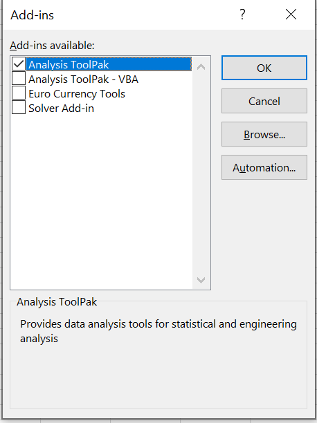
3d) Activate Excel’s Data Analysis add-in from the FILE >> OPTIONS >> ADD-INS menu.
Click Manage Excel Add-in and click the “Go..” button. Check “Analysis Toolpak” and this enables the “Data Analysis” function under the DATA tab.
RUN THE REGRESSION
4) The regression menu gives you some options. “Y Range” should be the salary column, while X Range should include the columns where the predictor fields are located.
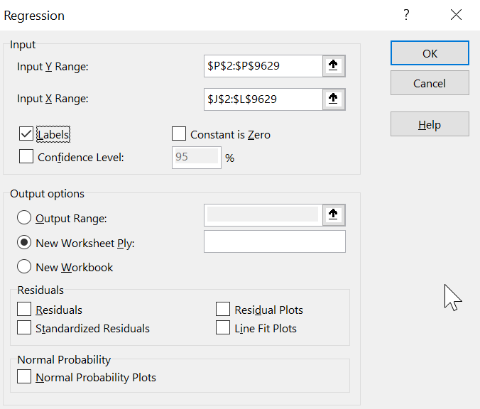
Click “OK” to run it on to a new sheet in the same workbook.
4a) R Square is a statistical measure of how well our data fits the model. The bigger the R square, the more goodness of fit. In our model, only 19% of the rows in the dataset fit the regression model which has Venue/Usage/Rest as independent variables.
We must add that R Square doesn’t indicate the correctness of the model. You better analyze R square together with the other alternative variables until you can get higher R-square values.
4b) Observations is the sample size (total rows) of the data.
4c) P-value (probability value) indicates probability of incorrectly rejecting the hypothesis. A p-value should be less than 0.05 (≤ 0.05) if you take the confidence interval 95%.
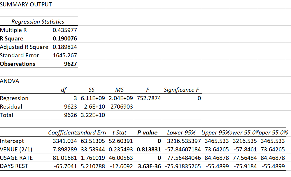
4d) According to results, Venue has a p-value of 0.813831446 which is higher than 0.05 confidence interval. Though, it doesn’t mean it has no effect on the salary. I recommend you replace the Venue factor with another metric and keep testing factors against the salary until you get a stronger R Square and smaller p-value.
4e) Rest days and usage rate factors have perfect p-values which are very close to zero and way smaller than 0.05.
4f) Intercept is the constant value when you want to set your salary prediction equation.
PREDICT A FUTURE SALARY
5) Calculate any player’s ideal salary and compare it to DK official salary given for today. So you can determine whether the player is undervalued or overvalued given his rest days, game-venue, and rest days.